QUESTION 01
What is a tree?
2 marksAnswer
A rooted tree is a hierarchical node structure with one root and one parent for every other node. Its underlying connected undirected graph has no cycle.

AR25 · I Year II Semester · Unit V — Trees and Graphs
QUESTION 01
A rooted tree is a hierarchical node structure with one root and one parent for every other node. Its underlying connected undirected graph has no cycle.
QUESTION 02
Trees represent hierarchical relationships such as directories, expression structure and search organisation.
The root has no parent. Children belong below a parent; siblings share a parent. A leaf has no children. A node’s degree is its number of children. A subtree contains a selected node and its descendants. This material measures height in edges: a leaf has height 0.
A root with two leaf children is perfect, full and complete. A chain is still a binary tree but can have height n - 1. A binary tree is not automatically a binary search tree: the search-order rule must be separately maintained.
A non-empty finite tree with n nodes has n - 1 parent-child edges. Traversing every node is O(n). Algorithms following a root-to-leaf path depend on height h, so the shape affects their work and recursive call depth.
Some texts count height in nodes rather than edges. State the convention before using a numerical formula instead of treating two consistent conventions as contradictory.
QUESTION 03
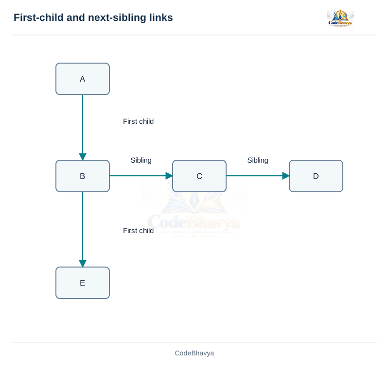
The left link identifies the first child; the right link identifies the next sibling. They are not both ordinary child links of the original tree.
QUESTION 04
A general rooted tree can be represented using at most two links per node without discarding its child order.
Suppose A has children B, C and D, and B has child E. Set A.left = B, B.right = C and C.right = D. Set B.left = E. D.right is NULL. The original root has no next sibling, so A.right is NULL.
C is a sibling of B, not an original child of B. Reading both links as original parent-child relations would misinterpret the general tree. The transformed pointer arrangement is binary in representation, but its semantic link meanings must remain clear.
A node needs two links regardless of how many children it has. There is no fixed child-array capacity to choose for every node. Iterating a node’s children means following the first-child link and then the sibling chain.
Creating one representation node per original node and linking each relationship once takes O(n) structural work and O(n) representation storage. Traversing a node’s k children via siblings takes O(k). This conversion is not a numeric BST insertion or balancing operation.
QUESTION 05
Preorder is root-left-right; inorder is left-root-right; postorder is left-right-root. The rules apply recursively to subtrees.
QUESTION 06
A traversal visits every tree node in a defined order.
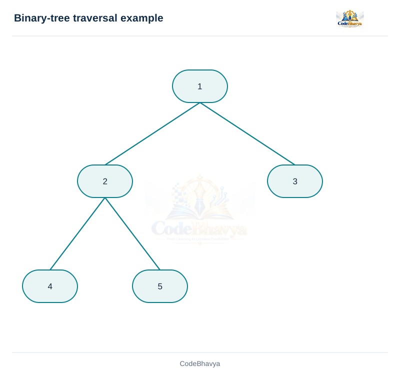
For root 1, children 2 and 3, and children 4 and 5 under node 2: preorder is 1 2 4 5 3; inorder is 4 2 5 1 3; postorder is 4 5 2 3 1. The complete example prints these orders.
For inorder without recursion, use an explicit node-pointer stack. Push nodes while moving left. When no left node remains, pop and visit one, then move to its right subtree. Repeat while either the current node exists or the stack is non-empty. The stack replaces the pending recursive calls.
Preorder can describe a parent before descendants. Postorder is useful when children must be handled before a parent, including tree destruction. Inorder gives increasing keys for a BST with its stated ordering policy, but not for every arbitrary binary tree.
Each node is visited once, so time is O(n). Recursive call depth is O(h), where h is tree height; it becomes O(n) for a chain. An explicit traversal stack has the corresponding height-dependent storage. A NULL root produces no values.
/* CodeBhavya | Data Structures AR25 | Learning example */
#include <stdio.h>
struct Node { int key; struct Node *left, *right; };
void preorder(const struct Node *p) { if (p != NULL) { printf("%d ", p->key); preorder(p->left); preorder(p->right); } }
void inorder(const struct Node *p) { if (p != NULL) { inorder(p->left); printf("%d ", p->key); inorder(p->right); } }
void postorder(const struct Node *p) { if (p != NULL) { postorder(p->left); postorder(p->right); printf("%d ", p->key); } }

int main(void)
{
    struct Node n4 = {4, NULL, NULL}, n5 = {5, NULL, NULL};
    struct Node n2 = {2, &n4, &n5}, n3 = {3, NULL, NULL}, root = {1, &n2, &n3};
    printf("Preorder: "); preorder(&root); putchar('\n');
    printf("Inorder: "); inorder(&root); putchar('\n');
    printf("Postorder: "); postorder(&root); putchar('\n');
    return 0;
}The example uses values in the code.
Preorder: 1 2 4 5 3
Inorder: 4 2 5 1 3
Postorder: 4 5 2 3 1QUESTION 07
Every key in a node’s left subtree is smaller and every key in its right subtree is larger. This example rejects duplicate insertions.
QUESTION 08
A BST combines a binary-tree shape with an ordering rule that guides search, insertion and deletion.
A BST interface can create an empty tree, search a key, insert a new key, remove a key and traverse or destroy the tree. The interface should define duplicate handling and how absence or allocation failure is reported.
For root 50, left child 30 and right child 70, searching 40 first moves left. If 30 has right child 40, the next move reaches it. The comparisons exclude the opposite subtree because all its keys lie on the wrong side of the BST ordering rule.
Inserting sorted keys into an ordinary unbalanced BST can make a chain. A basic BST does not automatically maintain a logarithmic height. Other duplicate policies can be valid, but must be consistent with searching, insertion and deletion.
A search follows at most one root-to-leaf path, so it takes O(h) time. A reasonably balanced shape has h = O(log n); worst-case height is O(n). An iterative search needs O(1) auxiliary space. Inorder traversal visits all n keys in sorted order under the stated policy.
/* CodeBhavya | Data Structures AR25 | Learning example */
#include <stdio.h>
#include <stdlib.h>
struct Node { int key; struct Node *left, *right; };
struct Node *insert(struct Node *root, int key, int *ok)
{
    if (root == NULL) {
        struct Node *node = malloc(sizeof *node);
        if (node == NULL) { *ok = 0; return NULL; }
        node->key = key; node->left = node->right = NULL; return node;
    }
    if (key < root->key) { root->left = insert(root->left, key, ok); }
    else if (key > root->key) { root->right = insert(root->right, key, ok); }
    return root;
}
const struct Node *search(const struct Node *root, int key)
{
    while (root != NULL && root->key != key) { root = key < root->key ? root->left : root->right; }
    return root;
}
struct Node *remove_key(struct Node *root, int key)
{
    if (root == NULL) { return NULL; }
    if (key < root->key) { root->left = remove_key(root->left, key); }
    else if (key > root->key) { root->right = remove_key(root->right, key); }
    else {
        if (root->left == NULL) { struct Node *next = root->right; free(root); return next; }
        if (root->right == NULL) { struct Node *next = root->left; free(root); return next; }
        struct Node *successor = root->right;
        while (successor->left != NULL) { successor = successor->left; }
        root->key = successor->key;
        root->right = remove_key(root->right, successor->key);
    }
    return root;
}
void inorder(const struct Node *root)
{
    if (root != NULL) { inorder(root->left); printf("%d ", root->key); inorder(root->right); }
}
void destroy(struct Node *root)
{
    if (root != NULL) { destroy(root->left); destroy(root->right); free(root); }
}

int main(void)
{
    struct Node *root = NULL; int ok = 1;
    int keys[7] = {50, 30, 70, 20, 40, 60, 80};
    for (int i = 0; i < 7; ++i) {
        root = insert(root, keys[i], &ok);
        if (!ok) { destroy(root); puts("Allocation failed"); return 1; }
    }
    printf("Search 40: %s\n", search(root, 40) != NULL ? "Found" : "Not found");
    root = remove_key(root, 20); root = remove_key(root, 30); root = remove_key(root, 50);
    inorder(root); putchar('\n'); destroy(root); root = NULL;
    return 0;
}The example uses values in the code.
Search 40: Found
40 60 70 80Insert 50, 30, 70, 20, 40, 60, 80 into an empty BST. Use one visit for each non-null node examined. Search for 65, which is absent.
| Node visited | Comparison | Next position |
|---|---|---|
| 50 | 65 > 50 | Right child: 70 |
| 70 | 65 < 70 | Left child: 60 |
| 60 | 65 > 60 | Right child: NULL |
The null link means there is no further candidate. Return “not found”; do not read a key through a null pointer. Searching for 60 follows the same first two moves and succeeds at the third node.
Now insert the same keys in sorted order: 20, 30, 40, 50, 60, 70, 80. In an ordinary BST, each new key becomes a right child, so searching for 80 visits all seven nodes. In the earlier tree it visits only 50, 70 and 80.
Therefore the insertion order affects the tree shape. The example BST does not balance itself. Its search follows one path: short paths give fast searches, while a chain can require O(n) visits. A traversal is different: inorder traversal must visit all n nodes even when the tree is balanced.
The ordering rule applies to whole subtrees. Suppose 30 is the left child of 50 and 55 is the right child of 30. Although 55 is greater than its parent 30, it is still in the left subtree of 50 and violates the BST rule. A search for 55 would move right from 50 and could miss it.
The following are topic matches from the supplied papers. Marks are their printed allocations, separate from the practice answer badge.
Illustrate search in a binary search tree.
Paper DS01 · page 1Define a binary search tree.
Paper DS03 · page 1Explain binary search trees.
Paper DS04 · page 1QUESTION 09
At the missing child link reached by repeatedly comparing the key from the root. A new ordinary insertion creates a leaf.
QUESTION 10
Insertion finds the key’s permitted location while preserving the ordering rule.
Insert 50, 30, 70, 20 and 40. The first key becomes root. 30 goes left of 50 and 70 right. 20 goes left of 30; 40 goes right of 30. Inorder traversal is 20, 30, 40, 50, 70.
Set a new node’s child links to NULL. If allocation fails, leave the existing tree valid and report failure. A recursive implementation must return the possibly changed subtree root and the caller must store it, including the first insertion into an empty tree.
The same key set can form different shapes for different insertion orders. The values are ordered logically by comparisons, not necessarily by the physical addresses of the nodes. This operation does not perform AVL or red-black balancing.
Insertion follows one path of height h, giving O(h) comparisons plus node allocation. Worst case is O(n); a balanced shape gives O(log n). Recursive extra call space is O(h), while an iterative implementation can keep fixed working pointers.
/* CodeBhavya | Data Structures AR25 | Learning example */
#include <stdio.h>
#include <stdlib.h>
struct Node { int key; struct Node *left, *right; };
struct Node *insert(struct Node *root, int key, int *ok)
{
    if (root == NULL) {
        struct Node *node = malloc(sizeof *node);
        if (node == NULL) { *ok = 0; return NULL; }
        node->key = key; node->left = node->right = NULL; return node;
    }
    if (key < root->key) { root->left = insert(root->left, key, ok); }
    else if (key > root->key) { root->right = insert(root->right, key, ok); }
    return root;
}
const struct Node *search(const struct Node *root, int key)
{
    while (root != NULL && root->key != key) { root = key < root->key ? root->left : root->right; }
    return root;
}
struct Node *remove_key(struct Node *root, int key)
{
    if (root == NULL) { return NULL; }
    if (key < root->key) { root->left = remove_key(root->left, key); }
    else if (key > root->key) { root->right = remove_key(root->right, key); }
    else {
        if (root->left == NULL) { struct Node *next = root->right; free(root); return next; }
        if (root->right == NULL) { struct Node *next = root->left; free(root); return next; }
        struct Node *successor = root->right;
        while (successor->left != NULL) { successor = successor->left; }
        root->key = successor->key;
        root->right = remove_key(root->right, successor->key);
    }
    return root;
}
void inorder(const struct Node *root)
{
    if (root != NULL) { inorder(root->left); printf("%d ", root->key); inorder(root->right); }
}
void destroy(struct Node *root)
{
    if (root != NULL) { destroy(root->left); destroy(root->right); free(root); }
}

int main(void)
{
    struct Node *root = NULL; int ok = 1;
    int keys[7] = {50, 30, 70, 20, 40, 60, 80};
    for (int i = 0; i < 7; ++i) {
        root = insert(root, keys[i], &ok);
        if (!ok) { destroy(root); puts("Allocation failed"); return 1; }
    }
    printf("Search 40: %s\n", search(root, 40) != NULL ? "Found" : "Not found");
    root = remove_key(root, 20); root = remove_key(root, 30); root = remove_key(root, 50);
    inorder(root); putchar('\n'); destroy(root); root = NULL;
    return 0;
}The example uses values in the code.
Search 40: Found
40 60 70 80QUESTION 11
The target has zero children, one child or two children. The two-child case uses a suitable predecessor or successor replacement.
QUESTION 12
BST deletion must remove the target while preserving every subtree’s ordering relationship.
The right-subtree minimum is greater than every key in the left subtree and no larger than the remaining right-subtree keys. It has no left child, so deleting its old node reduces to a simpler case. Do not copy a whole node object including its link pointers as though that were only a key replacement.
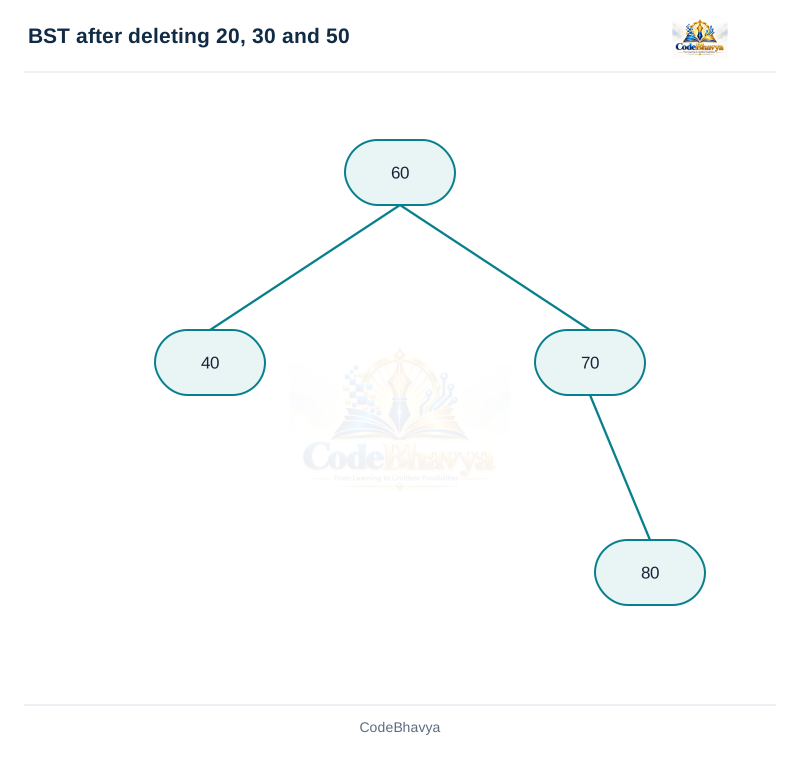
The demonstration builds 50, 30, 70, 20, 40, 60, 80. It deletes 20 as a leaf, 30 as a one-child node and 50 as a two-child root. The final inorder sequence is 40, 60, 70, 80.
Deleting the root can change the root pointer. Removing the only node makes the tree empty. Free exactly the removed node and keep no usable alias to it. A missing-key deletion is a normal unsuccessful operation.
Search and successor location follow paths bounded by tree height, giving O(h) time. Worst case is O(n), not unconditionally logarithmic. Recursive deletion uses O(h) call space. Destroy all remaining owned nodes when finished.
/* CodeBhavya | Data Structures AR25 | Learning example */
#include <stdio.h>
#include <stdlib.h>
struct Node { int key; struct Node *left, *right; };
struct Node *insert(struct Node *root, int key, int *ok)
{
    if (root == NULL) {
        struct Node *node = malloc(sizeof *node);
        if (node == NULL) { *ok = 0; return NULL; }
        node->key = key; node->left = node->right = NULL; return node;
    }
    if (key < root->key) { root->left = insert(root->left, key, ok); }
    else if (key > root->key) { root->right = insert(root->right, key, ok); }
    return root;
}
const struct Node *search(const struct Node *root, int key)
{
    while (root != NULL && root->key != key) { root = key < root->key ? root->left : root->right; }
    return root;
}
struct Node *remove_key(struct Node *root, int key)
{
    if (root == NULL) { return NULL; }
    if (key < root->key) { root->left = remove_key(root->left, key); }
    else if (key > root->key) { root->right = remove_key(root->right, key); }
    else {
        if (root->left == NULL) { struct Node *next = root->right; free(root); return next; }
        if (root->right == NULL) { struct Node *next = root->left; free(root); return next; }
        struct Node *successor = root->right;
        while (successor->left != NULL) { successor = successor->left; }
        root->key = successor->key;
        root->right = remove_key(root->right, successor->key);
    }
    return root;
}
void inorder(const struct Node *root)
{
    if (root != NULL) { inorder(root->left); printf("%d ", root->key); inorder(root->right); }
}
void destroy(struct Node *root)
{
    if (root != NULL) { destroy(root->left); destroy(root->right); free(root); }
}

int main(void)
{
    struct Node *root = NULL; int ok = 1;
    int keys[7] = {50, 30, 70, 20, 40, 60, 80};
    for (int i = 0; i < 7; ++i) {
        root = insert(root, keys[i], &ok);
        if (!ok) { destroy(root); puts("Allocation failed"); return 1; }
    }
    printf("Search 40: %s\n", search(root, 40) != NULL ? "Found" : "Not found");
    root = remove_key(root, 20); root = remove_key(root, 30); root = remove_key(root, 50);
    inorder(root); putchar('\n'); destroy(root); root = NULL;
    return 0;
}The example uses values in the code.
Search 40: Found
40 60 70 80The following are topic matches from the supplied papers. Marks are their printed allocations, separate from the practice answer badge.
Give BST deletion algorithm with an example.
Paper DS03 · page 2Give BST deletion algorithm.
Paper DS06 · page 1QUESTION 13
A graph G = (V, E) consists of vertices and edges describing relationships. Edges may be directed or undirected according to the model.
QUESTION 14
Graphs represent general connections rather than a single rooted hierarchy.
Adjacent vertices share a suitable edge. A path follows successive edges. A cycle returns to its starting vertex through the stated path convention. In an undirected graph, degree counts incident edges with loops treated by the chosen convention. A directed graph separates in-degree and out-degree.
Cities can be vertices and flights directed edges. A flight from city 2 to city 3 does not imply a return flight unless a separate edge is supplied. If time or price matters, store it as a weight with a defined meaning.
A finite connected undirected acyclic graph is a tree. A graph in general can contain cycles and disconnected components. Traversal therefore needs a visited record; merely following neighbours without one can revisit vertices indefinitely.
The representation controls adjacency tests and neighbour enumeration. An adjacency matrix uses O(V²) space, while adjacency lists use O(V + E) space for the usual representation. The ADT should specify edge direction, duplicate-edge and weight rules.
The following are topic matches from the supplied papers. Marks are their printed allocations, separate from the practice answer badge.
Define a graph.
Paper DS03 · page 1QUESTION 15
For an unweighted simple graph, entry [u][v] indicates whether the edge from u to v exists. An undirected matrix is symmetric.
QUESTION 16
An adjacency matrix stores pairwise edge information; an adjacency list stores each vertex’s neighbours.
A V-by-V array allows a direct O(1) edge test for valid indices. It uses O(V²) storage even for a sparse graph. Listing one vertex’s neighbours scans its row and can require O(V) work. A weighted representation needs a clear absent-edge encoding that does not confuse a valid zero weight with absence.
Each vertex stores its adjacent vertices or outgoing edges. Space is O(V + E), with an undirected edge ordinarily represented at both endpoints. Enumerating neighbours takes work proportional to the stored degree. A basic unsorted-list edge lookup can require O(degree) comparisons.
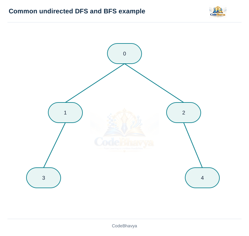
For undirected edges 0–1, 0–2, 1–3 and 2–4, row 0 has ones at columns 1 and 2. The list for 0 is [1, 2]. The list for 1 includes 0 and 3. Directed edges would not automatically create these reverse entries.
Use a matrix when graphs are small or dense and frequent edge tests matter. Lists suit sparse graphs and neighbour-driven traversal. State whether self-loops, duplicates and weights are supported rather than assuming every representation means the same graph model.
DFS or BFS using lists is O(V + E). With a matrix, scanning V possible neighbours for every visited vertex gives O(V²) in a full traversal. Quoting O(V + E) without identifying representation can therefore misdescribe a matrix implementation.
The following are topic matches from the supplied papers. Marks are their printed allocations, separate from the practice answer badge.
Give an example of an adjacency list of a graph.
Paper DS01 · page 1QUESTION 17
It explores one unvisited branch as far as possible before returning to another pending branch. Recursion or an explicit stack can manage the pending work.
QUESTION 18
DFS records visited vertices and explores neighbours deeply before backtracking.
For undirected edges 0–1, 0–2, 1–3 and 2–4, start at 0 and examine neighbour indices in ascending order. The DFS order is 0, 1, 3, 2, 4. From 1 it explores 3 before returning to 0 and considering 2.
Mark a vertex before exploring its outgoing neighbours. This prevents cycles from repeatedly recursing into an already discovered vertex. The same graph can have different valid DFS orders when start or neighbour order changes.
DFS supports reachability, component exploration and more specialised graph analyses. Detecting cycles or computing a topological order requires additional logic; a simple visited-only traversal should not be claimed to perform those tasks automatically.
With adjacency lists, a full traversal processes V vertices and their stored edges, giving O(V + E) time. The supplied program uses a matrix and scans a whole row per visited vertex, giving O(V²). Visited storage and worst-case recursion depth are O(V). The fixed example graph is connected, so one starting call reaches every vertex.
/* CodeBhavya | Data Structures AR25 | Learning example */
#include <stdio.h>
#define V 5
static const int graph[V][V] = {
    {0,1,1,0,0}, {1,0,0,1,0}, {1,0,0,0,1}, {0,1,0,0,0}, {0,0,1,0,0}
};
void dfs(int vertex, int visited[V])
{
    visited[vertex] = 1; printf("%d ", vertex);
    for (int next = 0; next < V; ++next) {
        if (graph[vertex][next] && !visited[next]) { dfs(next, visited); }
    }
}
void bfs(int start)
{
    int visited[V] = {0}, queue[V], front = 0, rear = 0;
    visited[start] = 1; queue[rear++] = start;
    while (front < rear) {
        int vertex = queue[front++]; printf("%d ", vertex);
        for (int next = 0; next < V; ++next) {
            if (graph[vertex][next] && !visited[next]) { visited[next] = 1; queue[rear++] = next; }
        }
    }
}

int main(void)
{
    int visited[V] = {0};
    printf("DFS: "); dfs(0, visited); putchar('\n');
    printf("BFS: "); bfs(0); putchar('\n');
    return 0;
}The example uses values in the code.
DFS: 0 1 3 2 4
BFS: 0 1 2 3 4The following are topic matches from the supplied papers. Marks are their printed allocations, separate from the practice answer badge.
Explain DFS with an example.
Paper DS03 · page 2Explain depth-first graph traversal with an example.
Paper DS04 · page 1Give DFS algorithm with an example.
Paper DS05 · page 1QUESTION 19
When it is enqueued. This prevents several neighbours from inserting the same vertex repeatedly.
QUESTION 20
BFS explores vertices in increasing edge distance from a starting vertex in an unweighted graph.
For edges 0–1, 0–2, 1–3 and 2–4, begin at 0. Enqueue 1 and 2 after processing 0. Process 1 and discover 3, then process 2 and discover 4. With ascending neighbour order, the output is 0, 1, 2, 3, 4.
The queue processes all earlier discovered vertices before later ones. Consequently all distance-one vertices are handled before distance-two vertices. A stack would instead promote a latest-discovered branch and give DFS-like behaviour.
BFS can record a predecessor and distance at discovery to obtain shortest paths measured in number of edges in an unweighted graph. This is not a universal least-cost algorithm for arbitrary weighted graphs. The demonstration prints traversal order only and does not claim to return a full path.
Adjacency-list BFS is O(V + E). The supplied matrix demonstration is O(V²) because each processed vertex scans V possible neighbours. Its queue and visited array need O(V) space. Marking at enqueue ensures each vertex enters the queue at most once per traversal.
/* CodeBhavya | Data Structures AR25 | Learning example */
#include <stdio.h>
#define V 5
static const int graph[V][V] = {
    {0,1,1,0,0}, {1,0,0,1,0}, {1,0,0,0,1}, {0,1,0,0,0}, {0,0,1,0,0}
};
void dfs(int vertex, int visited[V])
{
    visited[vertex] = 1; printf("%d ", vertex);
    for (int next = 0; next < V; ++next) {
        if (graph[vertex][next] && !visited[next]) { dfs(next, visited); }
    }
}
void bfs(int start)
{
    int visited[V] = {0}, queue[V], front = 0, rear = 0;
    visited[start] = 1; queue[rear++] = start;
    while (front < rear) {
        int vertex = queue[front++]; printf("%d ", vertex);
        for (int next = 0; next < V; ++next) {
            if (graph[vertex][next] && !visited[next]) { visited[next] = 1; queue[rear++] = next; }
        }
    }
}

int main(void)
{
    int visited[V] = {0};
    printf("DFS: "); dfs(0, visited); putchar('\n');
    printf("BFS: "); bfs(0); putchar('\n');
    return 0;
}The example uses values in the code.
DFS: 0 1 3 2 4
BFS: 0 1 2 3 4The following are topic matches from the supplied papers. Marks are their printed allocations, separate from the practice answer badge.
Explain BFS with an example.
Paper DS03 · page 2QUESTION 21
BFS uses a FIFO queue; iterative DFS uses a stack. Recursive DFS uses pending function calls with stack-like order.
QUESTION 22
DFS and BFS both explore reachable vertices, but their pending-work order differs.
Both need a graph representation, a starting rule and visited tracking. Both must restart at unvisited vertices if the task requires every component. State neighbour order when giving one exact printed sequence.
It follows a branch before backtracking. On the common five-vertex example with ascending neighbours, it gives 0, 1, 3, 2, 4. An explicit stack or recursion keeps unfinished work. The maximum active depth can reach V.
It explores level by level using a queue. The same example gives 0, 1, 2, 3, 4. Mark on enqueue to avoid duplicate pending entries. It naturally supports unweighted edge-distance calculations when distances are recorded.
Both have O(V + E) time with standard adjacency lists and O(V²) with a matrix full traversal. Both can need O(V) auxiliary storage, although their practical pending-work patterns differ. The choice does not automatically reduce the representation’s own storage.
Use BFS for level-order reachability or shortest numbers of unweighted edges. DFS is useful for deep exploration and as a base for analyses that require entering and finishing vertices. Neither basic traversal performs all possible graph applications without additional state or rules.
| Feature | DFS | BFS |
|---|---|---|
| Pending work | Stack/calls | Queue |
| Exploration | Depth first | Level first |
| List time | O(V + E) | O(V + E) |
| Matrix time | O(V²) | O(V²) |
| Auxiliary space | O(V) worst case | O(V) worst case |
The following are topic matches from the supplied papers. Marks are their printed allocations, separate from the practice answer badge.
Compare BFS and DFS for a graph.
Paper DS01 · page 2Compare BFS and DFS with examples.
Paper DS02 · page 1Differentiate BFS and DFS.
Paper DS06 · page 1QUESTION 23
Create a graph, add or remove vertices or edges, test adjacency, enumerate neighbours and traverse according to the chosen graph model.
QUESTION 24
A graph ADT specifies vertices, edge relationships and permitted operations independently of a matrix or list implementation.
State whether vertices have fixed indices or external labels, whether edges are directed, and whether weights or duplicate edges are allowed. Define error results for invalid vertices and how a missing edge is represented.
A fixed matrix provides direct adjacency tests and simple bounds checks for a small graph. Adjacency lists store only present edges and suit sparse neighbour traversal. Removing a vertex requires updating incident edges and any index mapping; it is not just deleting one display label.
An edge should represent a well-defined relation. Friendship may be undirected while following an account may be directed. Travel distance and fare are different weights. A DFS or BFS traversal answers reachability questions, but a particular application may require additional algorithmic steps.
The ADT alone does not promise every operation is constant time. In a matrix, a valid edge lookup is O(1); a whole neighbour row scan is O(V). Lists have degree-based scans and O(V + E) storage. Separate the logical contract from the chosen performance characteristics.
QUESTION 25
Each flight has an origin and destination. A reverse connection exists only when another supplied flight provides it.
QUESTION 26
Use vertices 1 New Delhi, 2 Mumbai, 3 Chennai, 4 Bangalore and 5 Kolkata. The ten supplied flights determine ten directed edges.
2→3, 3→2, 5→3, 3→4, 2→5, 5→2, 5→1, 1→4, 5→4 and 4→5. Flight numbers distinguish the source rows; the unweighted graph records the stated endpoint relationships.
Use rows as origins and columns as destinations in city-index order 1 through 5. A 1 records an outgoing connection; zero means that directed edge was not supplied. The table below is intentionally not made symmetric unless reverse flights actually appear.
There are ten 1 entries, matching the ten distinct supplied directed edges. Row 5 has four outgoing flights. Column 5 has incoming edges from cities 2 and 4. No self-flight is present, so the diagonal entries are zero.
A matrix stores 25 entries for these five cities. The adjacency lists store five vertex headers plus ten outgoing neighbour entries. General matrix space is O(V²); list space is O(V + E). No distance or fare is provided, so adding weights would invent information not present in the paper.
| Origin / destination | 1 | 2 | 3 | 4 | 5 |
|---|---|---|---|---|---|
| 1 | 0 | 0 | 0 | 1 | 0 |
| 2 | 0 | 0 | 1 | 0 | 1 |
| 3 | 0 | 1 | 0 | 1 | 0 |
| 4 | 0 | 0 | 0 | 0 | 1 |
| 5 | 1 | 1 | 1 | 1 | 0 |
The following are topic matches from the supplied papers. Marks are their printed allocations, separate from the practice answer badge.
Represent the supplied five-city flight network as a directed graph, adjacency matrix and adjacency list.
Paper DS03 · page 2